R for Biologists
A collection of episodes with videos, codes, and exercises for learning the basics
of the R programming language through examples.
Introduction to R
R and Unix

Beginnings
# ------------------------------------------------------------------
# File name: beginnings.R
#
# A line starting with # character is a comment line and is not interpreted by R
# Use comment lines liberally in your R scripts
# As you study these scripts, make sure to type each line in your copy of R
#
# Version: 2.1
# Authors: H. Kocak, University of Miami and B. Koc, Stetson University
# References:
# https://www.r-project.org
# ------------------------------------------------------------------

# R as a calculator
2+3.1

# Semicolon is a statement separator
2*3; 2/3

# R displays 7 digits by default. You can display more digits with options().
# More than 15 digits could be unreliable
# This is a global option; remains in effect until further notice
options(digits = 15)

# ^ for power
2/3; 2.1^3.1

# R has built-in mathematical constants and functions
2*pi
sin(2*pi)

# This is e
exp(1)

sqrt(2)

# Variables and their values are saved in the memory
# The assignment operators = or <- are equivalent. The right-hand-side
# is evaluated first and the result is assigned to the variable on the left.

# Variable names must start with a letter and can have letters, digits, underscore, and period.
# R distinguishes between upper and lower case
# Try to use suggestive, not cryptic, variable names

# x is a varible with value 2.1
x = 2.1

# To print the value of the variable x
x

# Same assignment as = in the previous statement
x <- 2.1
x

# plus_2 is another variable holding 2
plus_2 = 2.0

# Add the value of x and value of plus_2 and assign it as the new value of x
# old value of x is lost
x = x + plus_2


# Printing in R can be accomplished in three basic ways:

# simply type the variable name
x

# print(x) function: simply prints the value of x; its use sometimes necessary
# in loops and user-defined functions
print(x)

# cat() function concatenates strings, inside double quotes, and interpolated values of variables
cat("x =", x, "\n")
cat("root2 =", sqrt(2), "\n", "root3 =", sqrt(3), "\n")

# A variable can also hold a string in quotes
my_name = "Huseyin Kocak"
cat("My name is", my_name)

# You can quit R by
quit()
R Help

# ------------------------------------------------------------------
# File name: R_help.R
#
# R has readily accessible help facilities from the command line
# Below is an annotated summary of common help commands
# For more extensive information, see R Help
#
# Version: 2.1
# Authors: H. Kocak, University of Miami and B. Koc, Stetson University
# References:
# https://www.r-project.org
# ------------------------------------------------------------------

# To see a sequence of simple graphics pictures
demo(graphics)

# To see a sequence of 3D graphics
demo(persp)

# To list available demonstrations in base package of R
demo()

# To list all arithmetic operators in R
help(Arithmetic)

# To get help on the log function
help(log)

# To display R help on the plot() function
help(plot)

# Same as help(plot)
?plot

# To see example of the usage of plot function
example(plot)

# To list all R commands containing the string plot; could be too much info
help.search("plot")

# Same as help.search("plot")
??plot

# To get more help on the help() function
help()
Vectors

# ------------------------------------------------------------------
# File name: vectors.R
#
# R is efficient in computing with vector variables
# By default, a variable holding a single number is a vector of length 1
# Below is an annotated summary of common operations with vector variables
#
# Version: 2.1
# Authors: H. Kocak, University of Miami and B. Koc, Stetson University
# References:
# https://www.r-project.org
# ------------------------------------------------------------------

# R function c() combines (concatanes) values into a vector
x = c(1.5, -3.2, 0.45, 4.1, 10)
print(x)

# Entry of a vector can be addressed by its index, its position in the vector
# Unlike other programming languages, index of a vector in R starts from 1

# To print the first entry of x
print(x[1])

# To print the 4th entry of x
print(x[4])

# To change the value of the 4th entry of x to 7.6
x[4] = 7.6
print(x)

# Can add an entry to a vector
x[6] = 91
print(x)

# An entry of a vector can be deleted using -index
x = x[-6]
print (x)

# R function length() returns the number of entries of a vector
# There are numerous function for vectors; try, for example
# sort(), rev(), min(), mean(), sum(), prod()

length_of_x = length(x)
print(length_of_x)

# Arithmetic of vectors is done entry-wise
# + addition, - subtraction, * product, / division, %*% crossproduct

vector_1 = c(1.1, 2.3, 4.5)
vector_2 = c(-1, 1.2, 0.5)
vector_sum = vector_1 + vector_2
print(vector_sum)

# Vector entries can be strings or booleans
nucleotides = c("A", "C", "G", "T")
print(nucleotides)

# Vectors with patterns are useful. We will see a better way to generate them
x = c(0, 0.5, 1.0, 1.5, 2.0, 2.5, 3.0)
print (x)

squareRoot_x = sqrt(x)
print(squareRoot_x)
Sequences

# ------------------------------------------------------------------
# File name: sequences.R
#
# seq() function is used to generate a vector with specified patterns
# Below are common usages of seq() and some shortcuts for generating sequences
#
# Version: 2.1
# Authors: H. Kocak, University of Miami and B. Koc, Stetson University
# References:
# https://www.r-project.org
# ------------------------------------------------------------------

# To generate a sequence with fixed increments and assign it to variable x
x = seq(from = 0, to = 10, by = 0.5)
print(x)

# The construction above can be shorten as
x = seq(0, 10, 0.5)
print(x)

# The same sequence above can be generated by specifying the number of entries
x = seq(from = 0, to = 10, length = 21)
print(x)

# To generate a sequence with increment 1 (by = 1) can be shorten as
x = seq(0, 10)
print(x)

# The sequence above can be shorten further as
x = 0:10
print(x)

# : operator has higher predecence than the arithmetical operations.
# Note the difference in the two sequences below

sequence_1 = 0 : 10 - 2
print(sequence_1)

sequence_2 = 0 : (10 - 2)
print(sequence_2)
Script

# ------------------------------------------------------------------
# File name: script.R
#
# A simple R script to plot square root function
# The graph will be output to the screen in a separate graphics window
#
# To execute R commands in a file, type source("filename.R") at the propmt
# R looks for files in a "working directory"; type getwd() to find out this directory
# Use setwd() to set working directory. For example, if the file script_plot.R is in the
# /Users/hk/Documents/R_scripts directory, type
# setwd("/Users/hk/Documents/R_scripts/") then source("script.R")
# In Unix, you can start R from the directory containing your R scripts
#
# Version: 2.1
# Authors: H. Kocak, University of Miami and B. Koc, Stetson University
# References:
# https://www.r-project.org
# ------------------------------------------------------------------

x = seq(from = 0, to = 10, by = 0.5)
square_root_x = sqrt(x)

plot(x, square_root_x)
Graphics
Plot
# ------------------------------------------------------------------
# File name: plot_options.R
#
# plot() is a high-level R function that opens a new plotting window
# Here, we will show some basic options to plot() with a sequence of plots
# of square root function with increasing complexity
# Type ?plot to see details of basic options; you can see
# 657 available colores by typing colors()
#
# Version: 2.1
# Authors: H. Kocak, University of Miami and B. Koc, Stetson University
# References:
# https://www.r-project.org
# ------------------------------------------------------------------

x = seq(from = 0, to = 10, by = 0.5)
square_root_x = sqrt(x)

# Plot x-values vs. square_root_x values with default options
plot(x, square_root_x)

# To pause between plots
par(ask = TRUE)

# To add title
plot(x, square_root_x, main = "My First Plot")

# To add label to y-axis
plot(x, square_root_x, main = "My First Plot", ylab = "sqrt(x)")

# To set limits of y-axis
plot(x, square_root_x, main = "My First Plot", ylab = "sqrt(x)", ylim = c(0, 10))

# To add color
plot(x, square_root_x, main = "My First Plot", ylab = "sqrt(x)", ylim = c(0, 10),
                        col = "blue")

# To over strike with both plotting characters, pch, and connecting lines
plot(x, square_root_x, main = "My First Plot", ylab = "sqrt(x)", ylim = c(0, 10),
                        col = "blue", type = "o")

# To set the line type
plot(x, square_root_x, main = "My First Plot", ylab = "sqrt(x)", ylim = c(0, 10),
                        col = "blue", type = "o", lty = "dotted")

# To set plotting character
plot(x, square_root_x, main = "My First Plot", ylab = "sqrt(x)", ylim = c(0, 10),
                        col = "blue", type = "o", lty = "dotted", pch = 22)
Saving To File

# ------------------------------------------------------------------
# File name: saving_to_file.R
#
# Saving the plot of square root function to a png file
# You can also save a picture as a pdf file by using the
# pdf() function with .pdf file extension
#
# The file is saved in the current working directory of R
# Existing file with same name is overwritten
# The graph will not be output to the screen, so you should save
# after you get the desired picture
#
# Version: 2.1
# Authors: H. Kocak, University of Miami and B. Koc, Stetson University
# References:
# https://www.r-project.org
# ------------------------------------------------------------------

png("square_root_function.png", bg = "gray", width = 600, height = 600)

x = seq(from = 0, to = 10, by = 0.5)
square_root_x = sqrt(x)

plot(x, square_root_x, main ="Graph of Square root function", xlim = c(0, 10), ylim = c(0, 10),
      col = "red", type = "o")

dev.off()
Add Plot
# ------------------------------------------------------------------
# File name: add_to_plot.R
#
# plot() is a high-level plotting function that opens a new plotting window
# using low-level functions, one can add to the open plot
# some of the commonly used adding functions are:
# points(), lines(), abline(), legend(), text()
# Below, we will plot a function and add to plot
# its inverse function, a line, text, and a legend
#
# Version: 2.1
# Authors: H. Kocak, University of Miami and B. Koc, Stetson University
# References:
# https://www.r-project.org
# ------------------------------------------------------------------

t = seq(from = 0, to = 10, by = 0.5)

# To pause between plots
par(ask = TRUE)

plot (t, sqrt(2 * t), main = "Adding to Plot", sub = "A function and its inverse",
      xlab = "", ylab = "", xlim = c(0, 10), ylim = c(0, 10), pch = 16, type = "o")

# To add the inverse function
points(t, 0.5 * t * t, col = "red" , pch = 16, type = "o")

# To add the line with intercept = 0, slope = 1
abline(0, 1, col = "gray", lwd = 3, lty = "dashed")

# To add text
text(7, 7.3, "45-degree line", srt = 45)
legend("bottomright", legend = c("funtion", "inverse"), pch = 16, col = c("black", "red"))

# One can add graphs of mathematical functions using, for example:
# lines(curve(sin(x) + cos(x) + 5,  add = TRUE))
Curve Plotting
# ------------------------------------------------------------------
# File name: curve_plotting.R
#
# curve() is a high-level mathematical plotting function that opens a new plotting window
# Variable in the mathematical formula must be x
# Can add more graphs by setting add = TRUE
#
# Version: 2.1
# Authors: H. Kocak, University of Miami and B. Koc, Stetson University
# References:
# https://www.r-project.org
# ------------------------------------------------------------------

curve(sin(x), xlim = c(-4*pi, 4*pi), ylim = c(-2, 2), col = "red", ylab = "")

# To plot horizontal line using h
abline(h=0, lty= "dotted")

# To mark the origin
points(0, 0, pch = 3)

curve(cos(x),  col = "blue", add = TRUE)
curve(sin(x) + cos(x),  col = "purple", lwd = 3, add = TRUE)

title("sin(x) + cos(x)")

legend("bottomright", legend = c("sin(x)", "cos(x)", "sin(x) + cos(x)"),
        lty = 1, col = c("red", "blue", "purple"))
Multiple Plots
# ------------------------------------------------------------------
# File name: multiple_plots.R
#
# With the par() command can set the multi plot environment.
# mfcol = c(nr,nc) partitions the graphic window as a matrix of nr rows and nc columns,
# the plots are then drawn in columns.
# mfrow = c(nr,nc) partitions the graphic window as a matrix of nr rows and nc columns,
# the plots are then drawn in rows.
# You can get fancy partitions of the plotting window with layout() function
#
# Version: 2.1
# Authors: H. Kocak, University of Miami and B. Koc, Stetson University
# References:
# https://www.r-project.org
# ------------------------------------------------------------------

par(ask=TRUE)

# Prepare for 2x2 plots, to be filled by rows
par(mfrow = c(2, 2))

t = seq(0, 10, 0.2)
plot(t, sin(t))
curve(sinh(x), -5, 5)
curve(tan(x), n = 500, -5, 5)
curve(round(x), n = 500, -5, 5)

# Return to single plot
par(mfrow = c(1, 1))

curve(sin(x), -5, 5)
Time Temp
00 32.77
02 33.16
04 33.35
06 33.57
08 33.67
10 33.75
12 33.85
14 33.94
16 33.98
18 34.03
20 34.04
Plot the temps as a function of time. Is the temp leveling off? Why?
Extra credit: Can you set the clock to any prescribed time XY:WZ (hour:minute)?
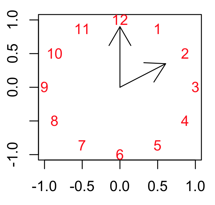
# clock by Hlynka
# Look up in the R manual the function arrows()
# Add title, beautify it as you please

plot(-1:1, -1:1,  type = "n",  xlab = "",  ylab = "" )
K = 12
text(exp(1i * 2 * pi * c(2:1,12:3) / K),  col = "red")
arrows( 0, 0, 0, 0.9)
arrows( 0, 0, 0.7*cos(pi/6), 0.7*sin(pi/6))
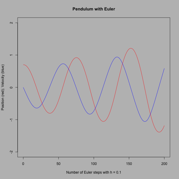
E(Θ , Θ') = (1/2)m(L^2)(Θ'^2) + mgL(1- cos(Θ)).
This Energy function is supposed to be conserved along
the solutions of the pendulum. Show this assertion by computing
dE/dt using the chain rule, keeping in mind that Θ and
Θ' depend on t, and the differential equations for pendulum.
Observe that dE/dt = 0, so it must be constant function of t.
Conditionals and Loops
If Else

# ------------------------------------------------------------------
# File name: if_else.R
#
# This code asks the user to enter a number.
# If the number is non-negative, it prints the sqrt of the number;
# otherwise, it exits with a message.
# Decision is accomplished with an if() else statement
#
# Version: 2.1
# Authors: H. Kocak, University of Miami and B. Koc, Stetson University
# References:
# https://www.r-project.org
# ------------------------------------------------------------------

cat("Please enter a number to compute its square root \n")

# To get input from keyboard (single item)
x = scan(nmax = 1, quiet = TRUE)

cat("The number you have entered is", x, "\n")

# Else must be on the same line as the closing brace of if
if(x >= 0) {
    cat("square root of", x, "is", sqrt(x), "\n")
} else {
    cat("Sorry, please enter a nonnegative number \n")
}

cat("Bye!. \n")
For
# ------------------------------------------------------------------
# File name: for_loops.R
#
# for loop in R iterates a block of statements with a counter running through
# values in a sequence. Syntax of for loop is:
# for (counter in sequence) {
# statements
# }
#
# Version: 2.1
# Authors: H. Kocak, University of Miami and B. Koc, Stetson University
# References:
# https://www.r-project.org
# ------------------------------------------------------------------
sequence = seq (1, 10)
for(counter in sequence) {
squared = counter * counter
cat("counter = ", counter, "\t", "squared = ", squared, "\n" )
}
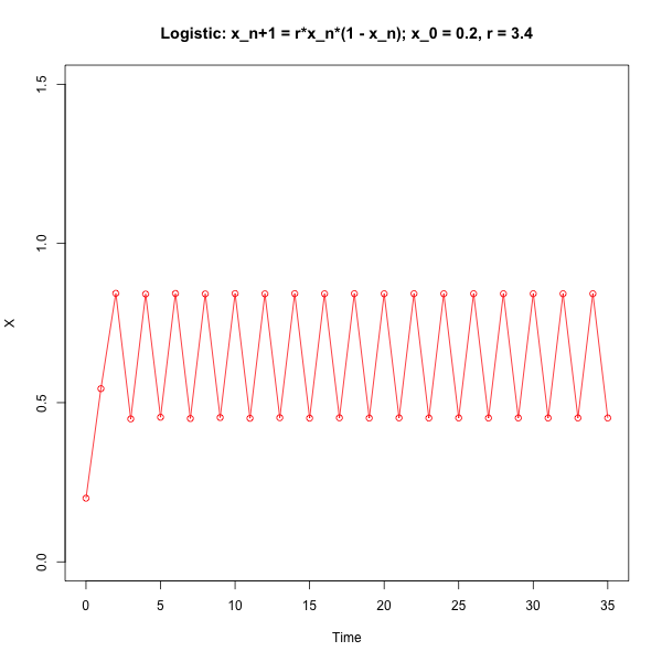
# In the following more complicated example of for loop, we will compute 10 generations of
# a population growing according to the discrete logistic model and save the
# population densities as a vector
cat("Densities of generations with discrete logistic growth model \n")
# Initialize vector holding population densities; x[1] = 0.2
x = 0.2
cat("generation =", 1, "\t", "population density =", x[1], "\n" )
# Growth rate
r = 2.45
number_of_generations = 10
for(i in 1:(number_of_generations - 1)) {
x[i+1] = r*x[i] * (1.0 - x[i])
cat("generation =", i+1, "\t", "population density =", x[i+1], "\n" )
}
# To see x as a vector
print (x)
While

# ------------------------------------------------------------------
# File name: while_loops.R
#
# while loop iterates a block of statements as long as a condition (boolean) remains true.
# Syntax of while loop is:
# while (boolean){
#	statements
# }
# break exits the loop
#
# Version: 2.1
# Authors: H. Kocak, University of Miami and B. Koc, Stetson University
# References:
# https://www.r-project.org
# ------------------------------------------------------------------

# To generate a table of numbers and their squares

counter = 1

while (counter <= 10){
   square = counter * counter
   cat("counter = ", counter, "\t", "square = ", square, "\n" )
   counter = counter + 1
}


# Newton-Raphson iteration for finding sqrt(2) with a specified tolerance
# x = starting value
# delta = absolute value of the difference between two consecutive iterates
# while performs Newton-Raphson iterates as long as delta remains greater than
# a desired tolerance

cat("Newton-Raphson iteration for computing sqrt(2) with a specified tolerance \n")
options(digits = 15)

x = 3.1
tolerance = 1e-8
cat("x =", x, "\t", "tolerance =", tolerance, "\n")

x_next = 0.5 * (x + 2/x)
delta = abs(x_next - x)
cat("x =", x_next, "\t", "delta =", delta, "\n")
x = x_next

while (delta > tolerance){
  x_next = 0.5 * (x + 2/x)
  delta = abs(x_next - x)
  cat("x =", x_next, "\t", "delta =", delta, "\n")
  x = x_next
}
Writing Functions
Writing Functions
# ------------------------------------------------------------------
# File name: writing_functions.R
#
# User-defined functions have the form
# name = function(parameters ){
#	statements
# return()
# }
# After sourcing this file, the functions herein will be loaded into memory.
# The first function just prints out my address. Usage: my_address()
# The second function computes and returns the Taylor series approximation of sin(x) to
# a specified number of terms. Usage: sine_series(0.5, 5) to compute the
# sin of 0.5 for 5 terms.
#
# Version: 2.1
# Authors: H. Kocak, University of Miami and B. Koc, Stetson University
# References:
# https://www.r-project.org
# ------------------------------------------------------------------

my_address = function(){
  cat("Huseyin Kocak\n")
  cat("Department of Computer Science\n")
  cat("University of Miami\n")
  cat("Coral Gables, FL 33146\n")
}

options(digits = 15)

sine_series = function(x, number_of_terms){
  sum = 0

  for(n in 0:(number_of_terms-1)){
    sum = sum + ( ((-1)^n) / factorial(2 * n + 1) ) * (x^(2 * n + 1) )
  }

  return(sum)
}
newtonFor_A = function(A, x, number_of_iterations)
to compute the square root of any positive number A.
#newton iteration for finding sqrt(2)
#parameters
# x = starting value
# number_of_iterations = number of iterations
#usage: newtonFor(3.1, 8)

#to get more digits use options(digits=15)

newtonFor = function(x, number_of_iterations){  #begin function
    print(x)
    for ( i in 1:number_of_iterations){    #index i will run from 1 to number_of_iterations
      x = 0.5*(x + 2/x)                    #replace old x with new value
      print (x)
    }                                      #end for
}                                          #end function
# This script is from R for Beginners, by E. Paradis.
# ricker function iterates the Ricker model, a difference equation for
# modeling the growth of a single population, and plots fifty generations
# for three values of parameter r.


ricker <- function(nzero, r, K=1, time=50, from=0, to=time)
{
N=0
N[1] <- nzero
for (i in 1:time) N[i+1] <- N[i]*exp(r*(1 - N[i]/K))
Time <- 0:time
plot(Time, N, type="o", xlim=c(from, to))
}


layout(matrix(1:3, 3, 1))
ricker(0.1, 1); title("Ricker model with r = 1")
ricker(0.1, 2); title("r = 2")
ricker(0.1, 3); title("r = 3")
Curve Fitting and Parameters
Curve Fitting

# ------------------------------------------------------------------
# File name: curve_fitting.R
#
# Linear Model function lm(y~x) computes the least square fit line to data points;
# y as a function of x. Type ?formula for help with legal formulas.
# lm() can also be used to fit nonlinear models where the parameters enter into model linearly.
#
# Version: 2.1
# Authors: H. Kocak, University of Miami and B. Koc, Stetson University
# References:
# https://www.r-project.org
# ------------------------------------------------------------------

# Fit a line to two data points; a good test of lm()
x2 = c(1, 2)
y2 = c(1.5, 2.5)

plot(x2, y2, main="Unique line through 2 points", xlim=c(0, 4), ylim = c(0, 4))

# Compute the least square line, save output in ls_fit_line
ls_fit_line = lm(y2 ~ x2)
print(ls_fit_line)

# Plot the least square line stored in ls_fit_line
abline(ls_fit_line, col="red")

# Print the vector containing intercept and slope the line
print(coef(ls_fit_line))

# Lots more info
print(summary(ls_fit_line))

par(ask=TRUE)

# Compute least-square line fit for 3 data points
x3 = c(1, 2, 3)
y3 = c(1.5, 2.5, 2.8)

plot(x3, y3, main="Best-fit line through 3 points", xlim=c(0, 4), ylim = c(0, 4))
fit3 = lm(y3 ~ x3)
abline(fit3, col = "red")
print(fit3)

# Lots more info about the fitness
print(summary(fit3))

# Compute the parabola through 3 data points

plot(x3, y3, main="Unique parabola through 3 points", xlim=c(0, 6), ylim = c(0, 6))
fit_parabola3 = lm(y3 ~ x3 + I(x3^2))
print(fit_parabola3 )
curve(coef(fit_parabola3)[1] + coef(fit_parabola3)[2]* x + coef(fit_parabola3)[3]*x^2,
      0, 6, col = "red", add=TRUE)

# Compute a best-fit parabola for 4 data points

x4 = c(1, 2, 3, 4)
y4 = c(1.5, 2.5, 2.8, 1.7)

plot(x4, y4, main="Best-fit parabola through 4 points", xlim=c(0, 6), ylim = c(0, 6))
fit_parabola4 = lm(y4 ~ x4 + I(x4^2))
print(fit_parabola4)
curve(coef(fit_parabola4)[1] + coef(fit_parabola4)[2]* x + coef(fit_parabola4)[3]*x^2,
      0, 6, col = "red", add=TRUE)

# Add the predicted points
points(x4, predict(fit_parabola4), col = "green")
Beetle
# ------------------------------------------------------------------
# File name: beetle_parameters.R
#
# Problem:
# Flour beetles with initial 112 individiuals are grown
# in a laboratory are counted daily for 15 days.
# Assuming that the beetle population grows according to the logistic differential
# equation (dy/dt) = ay + by^2, where y[t] is the population size at time t,
# estimate the values of the parameters a and b.
#
# Solution:
# Rewrite the differential equation as (dy/dt)/y = a + by so that r.h.s is linear in y
# Approximate the derivative with (y[t+h] - y[t])/h, here h=1,
# Compute  15  points, ((y[t+h] - y[t])/y[t], y[t]) and determine the best fit line.
# Intercept = a and slope = b.
#
# Version: 2.1
# Authors: H. Kocak, University of Miami and B. Koc, Stetson University
# References:
# https://www.r-project.org
# ------------------------------------------------------------------

# First, record the data and plot it daily count of beetles for 16 days

# Beetle count for 15 days
y = c(112, 152, 212, 258, 306, 309, 315, 310,
      298, 290, 303, 295, 311, 308, 299, 309)

# Time in days
t = seq(0, length(y)-1)

plot(t, y, main = "Daily beetle counts", type = "o", xlab = "days", ylab = "beetles")


# Remove the last data point (why?)
y_1 = y[-length(y)]

# To pause between plots
par(ask=TRUE)

# Create a rate vector and load it with computed rates
scaled_rate = 0

for(i in 1:(length(y)-1)) {
    scaled_rate[i] = (y[i+1] - y[i]) / y[i]
}

#print(rate)

# Plot 15 points and compute best line for them
plot(y_1, scaled_rate, col = "red", main = "Least square fit to scaled rates")

best_fit_line = lm(scaled_rate~y_1)       #compute line using lm() and save
abline(best_fit_line)                     #add the graph of the line
print(best_fit_line)                      #print intercept and slope of line

# If you know statistics, you can try the following commands for more information
# print(summary(best_fit_line))
# plot(best_fit_line)
(-1, 1.1), (0, 2.05), (1.8, -0.5).
Find the unique parabola y = a + bx + cx^2 passing through these three points.
Now write an R code that computes the averages of the data points and Phaser
points and prints out the difference between the two averages.
Time Temp
00 32.77
02 33.16
04 33.35
06 33.57
08 33.67
10 33.75
12 33.85
14 33.94
16 33.98
18 34.03
20 34.04
- Useful links:
- The R Project for Statistical Computing: Main Web site
This is the official Web site for R. You can download R for your computing platform. - R Reference card by M. Baggott and T. Short
- An Introduction to R
- R for Beginners by E. Paradis
- Using R for Scientific Computing`by K. Soetaert